crazygeology

The Flinn Diagram in Action

In a recent post we discussed the Flinn-Diagram. There it was possible to see that – depending on the orientation of the regional stress field – a rock can be deformed in several ways, but the deformation of a rock unit is of course not visible in a small outcrop. Therefor, we have to look at specific textures in smaller scales. Let’s think about it: in our example we deformed a cube. What would be ideal to use in real-life then? Easy, a mineral or geologic object with either a cubic or even better (better for the strain ellipsoid) a sphere-like appearance.

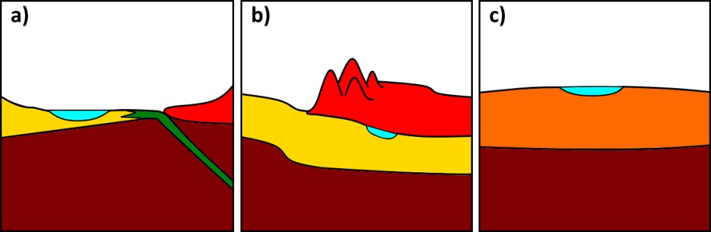
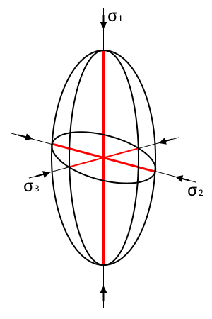
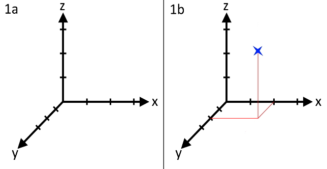
So, don’t let us waste any more time and begin. Imagine that we have a “raisin-cake” rock, meaning a rock with spheroid geological objects in them. What are these? Let’s just say that these are Ooids, small spheres of limestone. Another often proposed candidate is gas bubbles in volcanic rock, but I still have to see gas bubbles that did not show any deformation whatsoever. Anyway; a rock with some ooids and a mudstone-matrix gets formed in a shallow ocean environment (aka. Laguna; Fig. 1a). Later in time a subduction developed up to the point that the ooid-stone and other adjacent continental rocks get to the subduction zone, so that a thrust zone develops (Fig. 1b). Now some orogenesis occurs and our rock unit gets buried. Later the overlying rock units will be eroded, and our rock will be exposed at the surface again (Fig. 1c). Due to the local stress regime, our ooids will now be deformed, but how?

Fig. 1. Geotectonic evolution of our hypothetical example. The lagoon with the ooid-containing rock is marked in blue.

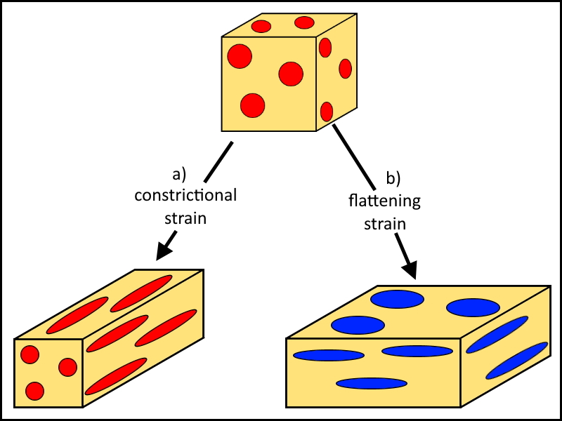
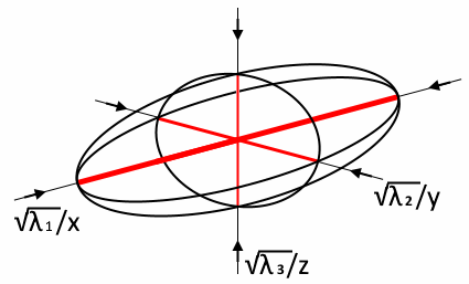
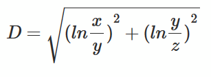
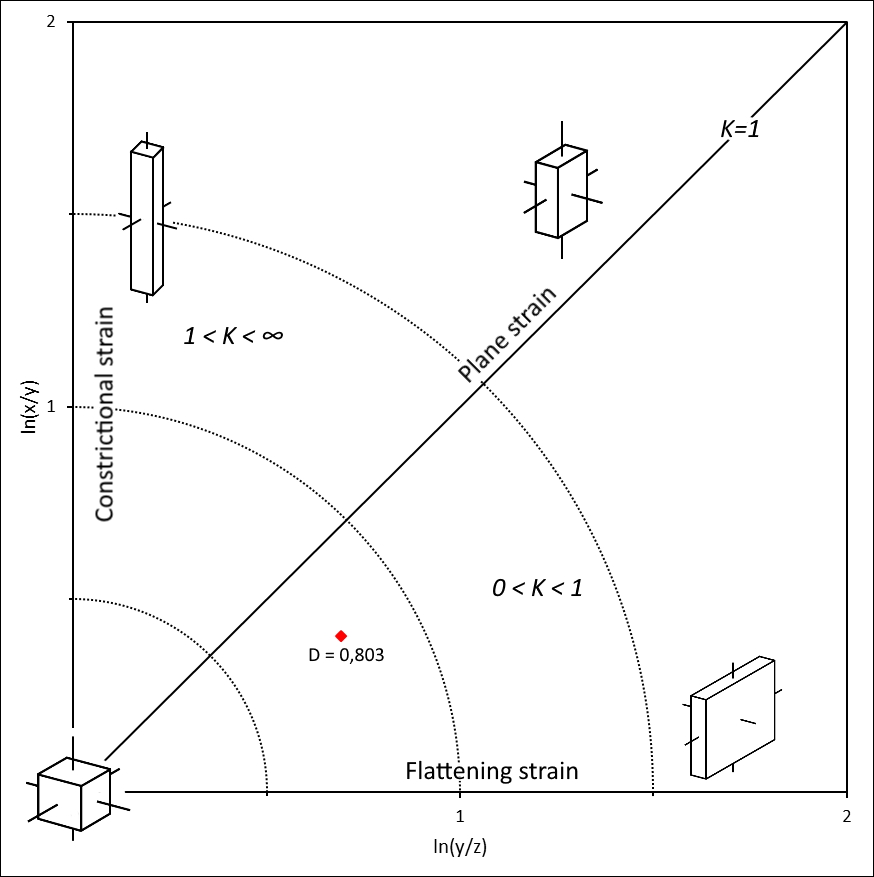
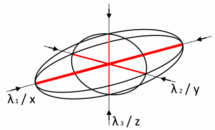
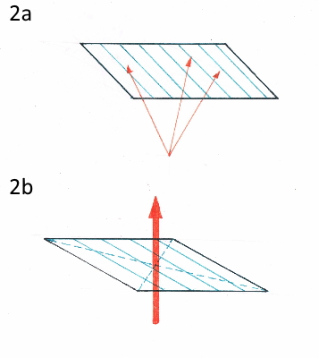
Let’s recap: Our strain model is basically bimodal with constrictional strain as one end member and flattening strain as another end member.

Therefore, if only constrictional strain is applied to our rock, our round ooids will deform to long cigars (Fig. 2a). If only flattening strain is applied to our rock, then we will get discus-like (or pancake-like) ooids (Fig. 2b). If you speak Polish, Czech, German or French there is a little trick here. Do you remember how we call stress ellipsoids if they appear flattened? Right, oblate ellipsoid. Now, how are these famous edible disks from Karlovy Vary called in the Czech language? Oplatka, correct! See, now you possibly know a new word and have a little trick to remind the shape of flattened geological objects.

Fig. 2. end members of tectonic deformation.

Back to our topic at hand. Now as we have applied our two extreme cases to our example, we can think of what would happen in an intermediary situation? Easy, right? Our ooids would both be flattened and elongated in one direction. However, this is all nice and good, but what do we do if we are in higher metamorphic conditions and the only stuff that we can see is gneiss? Well, for that we must introduce the terms lineation and foliation. Lineation (lineation –> linear –> line) describes whether or not minerals with one elongated axis are aligned in one direction. In the case of our ooids this means that if e.g. the longest axis of them is always oriented in N-S direction in the outcrop, our lineation is well developed and shows a N-S direction. Foliation (also called: schistosity) on the other hand (foliation –> foil –> planar object) means that objects show a good separation along parallel planes. Meaning: if you stack pancakes upon each other, they show perfect vertical foliation.

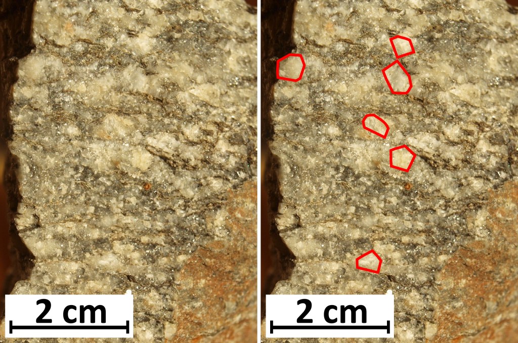
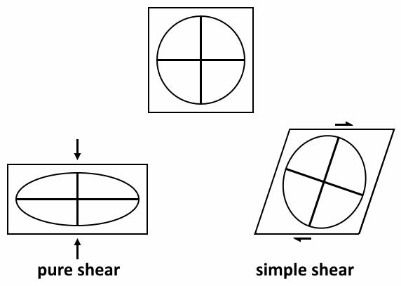
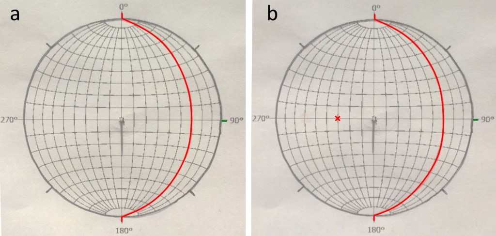
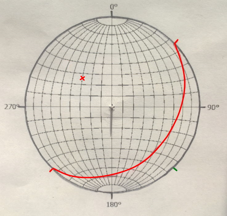
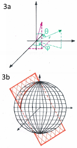
So, let’s apply this to a real-life rock, shall we? Let’s take a gneiss as an example. Assume that a sample of Freiberger gneiss shows a planar fabric of the mica minerals with a nearly horizontal orientation in the outcrop (Fig. 3).

Fig. 3. Planar fabric (foliation) of the gneiss.

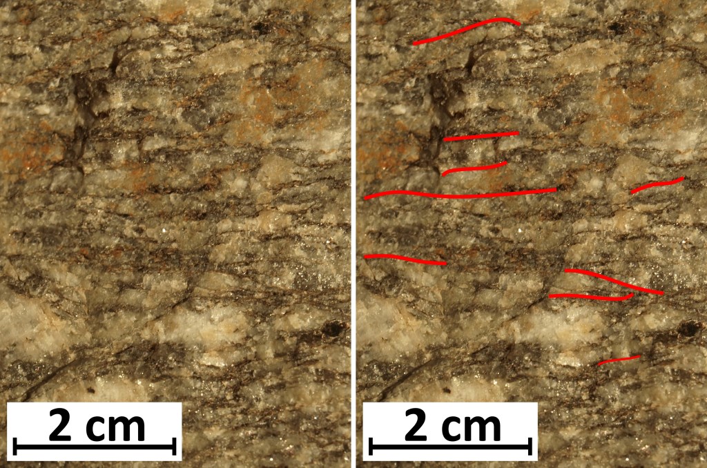
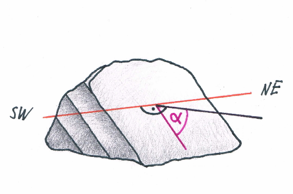
This is our pure shear component. In addition to that, our grains itself are all oriented in one direction, as can be seen on the “top” of the sample. Now we rotate our sample (meaning we hammer rocks away in our outcrop until we get what we want) to the face of the rock, that the elongated minerals are pointing to. Assume that in our sample the minerals are all oriented in NW-SE orientation. This is our lineation (Fig. 4).

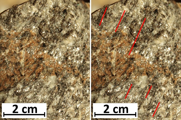
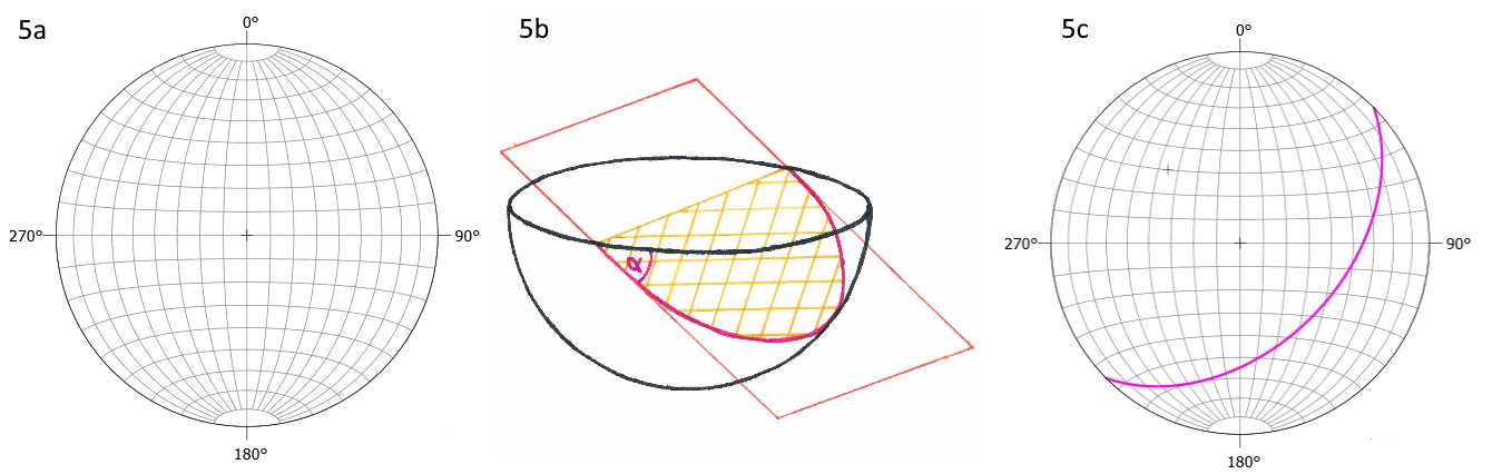
So, we only need to find (or hammer away rock) a surface with the strike values 45°-125° and a dip of 0° and look at this: our minerals appear nearly square-like (of course not completely square). This is our simple shear component.

Fig. 5. Plane perpendicular to the plane of the foliation. The linear of the lineation is the normal vector of the displayed plane.

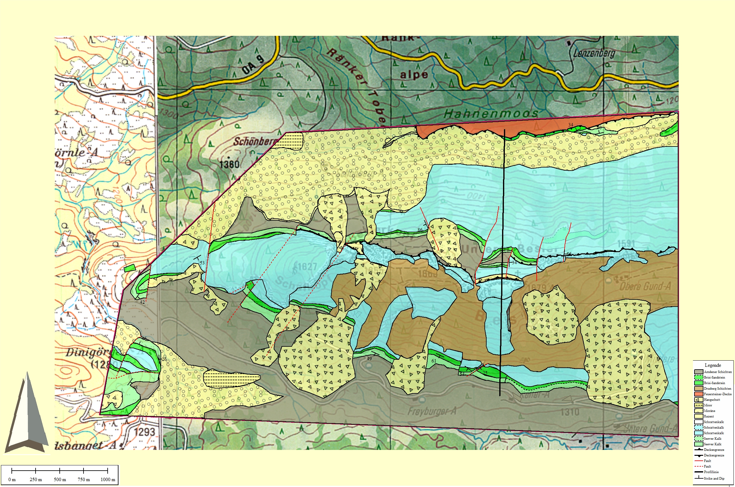
What we now cannot really determine from this data alone is whether our flattening strain dominated over our constrictional strain or vice versa. We could determine that if we were able to find e.g. deformed garnets in our sample where we could measure the different axis and place the value in the Flynn-Diagram accordingly. Now we look at a map of Europe (Fig. 6) and what do we see there? Our sample lies in the zone of the variscan metamorphic zone with several thrust zones that strike roughly from NE to SW.

Fig. 6 tectono-geologic map of Europe with variscan orogens marked. The red star marks the position of the sample. Map based on Leveridge & Hartley (2006).

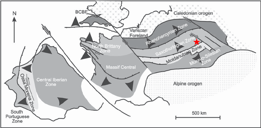
Does this fit with our observations? Indeed, it does! The overlaying rock provided simple shear, while the constrictional SE-NW oriented stress regime provided simple shear. If you are further interested in this topic, I highly advise you to look at this instagram post of Prof. John Encarnacion.

Source

Leveridge, B. & Hartley, A (2006). The Variscan Orogeny: the development and deformation of Devonian/Carboniferous basins in SW England and South Wales The Variscan of SW England. In: The Geology of England and Wales.

The Flinn diagram

In the previous post we covered the basics of stress and strain, but these alone are nothing. We need some examples! So; what are these? Obviously, I could talk about folds and faults now, but that is boring. Instead, let me introduce you to the Flynn diagram. We can use this in combination with our strain ellipsis to evaluate deformation regimes and therefor gather evidences for the development of a specific tectonic regime. Sounds interesting? Ok then; let’s go!

First a small reminder. What is the strain ellipsis? Well, the strain ellipsoid (Fig. 1) is the representation of the shape that a perfectly spherical grain would take if it was put in a defined stress regime. By convention the x-axis is always the axis of biggest elongation, while the z-axis gets the least elongated (meaning; in relation to the previously existing sphere it shrinks).

Fig.1: a representation of the strain ellipsoid

In order to illustrate the whole diagram to you, I will give you an example. Let’s say we find a rock with a bunch of ellipsoidal grains in it. In order to use the diagram, we now have to measure the length of the axes of the grains in our sample. (That means, that we have to note the orientation of the sample in the field before we even think about our hammer. Why? Well, because we want to determine the orientation of the stress field!)
For our specific example the x-axis shows a length of 3 cm, the y-axis shows a length of 2 cm and the z-axis shows a length of 1 cm. Now, let’s think a moment. What would happen, if we would change these values? Maybe, let’s say make it so that y=x or y=z. Our ellipsoid would change its form, correct? Indeed; these would be completely different shapes that we would be able to see. Therefor, in order to classify these different shapes some parameters together with a diagram were thought of; the Flinn diagram (Unfortunately I was not able to track down the original source publication for that, so yeah; you will have to deal with that. If you know of the first instance, where that diagram popped up, please notice me!). In order to use that diagram, we first have to introduce a new parameter; K. This parameter is defining the style of strain, meaning: the shape that the ellipsoid takes. K is calculated with:

Now, there is a little thing that I have to highlight here. In many publications (and also up to this point in the introduction) you can see that e.g. λ1 is used similar to x. This is actually wrong, if one wants to use proper terminology, but it does not matter here (see this post coming soon for explanation).

As you can imagine, different lengths of the axes result in different shapes. With that knowledge we can now construct the Flinn-diagram. In the origin point sits an undeformed sphere. This sphere now gets deformed, resulting in a value for K. That K-value functions as the slope of a specific function (see further down) in the diagram. Therefore, the values of ln(y/z) plot on the x-Axis in the Flinn-diagram, whereas the values of ln(x/y) plot on the y-axis. In addition to that, the Flinn diagram also contains the D-value. This value classifies the amount of strain; the ellipsoidicity (meaning how far away the ellipsoid is away from a perfect sphere) of our deformed grain. D is calculated with:

and represents the distance from the origin (meaning: perfect sphere) to your data point in the diagram. With all these values, we can now construct our Flinn-diagram (Fig. 2).

Fig. 2 The Flinn-diagram. Note that the red aquare notes our example that is described in text. As for visualisation: Imagine these cuboids as actually being spheres/ellipsoids. So, why did I draw cuboids? Well, because, screw drawing ellipsoids!

If you now take a look at the diagram, it won’t come as a surprise now if I tell you that the diagram can be differentiated into several sectors. These are based on the values for K:

K –> ∞	axially symmetric extension: x >>> y = z	the objects appear in a pencil-like shape and plot near the y-axis
∞ > K > 1	Constrictional strain: x > y ≥ z	the ellipsoids are elongated mainly along the x-axis, they look like cigars (so-called prolate ellipsoid)
K = 1	plane strain deformation: x > y > z	all deformation happens in one (mathematical) plane, that is perpendicular to y. The y-axis does not change in its length
1 > K > 0	Flattening strain: x ≥ y > z	ellipsoids get flattened down mainly along the z-axis, they look like thick pancakes (so-called oblate ellipsoid)
K –> 0	axially symmetric flattening: x = y >>> z	objects get extremely flattened only along the z-axis

Tab. 1 range of values that K can occupy.

As you can imagine, the K-value as presented in the table (Tab. 1) only represents the theoretical shape that can be reached in the end. As how pronounced that shape is, that is determined by the D-value. In our case the D has a value of 0,803, meaning that our grain is relatively similar to a sphere. The stress regime therefor has been relatively low for that grain.

So, why do we need all that? Well, think back about the different types of shear. There was “pure shear” and “simple shear”, right? Now, let’s look at the Flinn-diagram. Do you think one can produce pancake-shaped ellipsoids when only simple shear is applied to a rock with uniformal grains to it? Nah, I don’t think so either, but with pure shear, that would work perfectly, right?
As a result, we can use the shape of deformed mineral grains to trace that back tectonic regimes. Especially metamorphic rocks are awesome for that. We call these tectonites, which will be covered in another post (coming soon).

Ressources
Rey, Patrice: Strain and Strain Analysis. In: Structural Geology. URL
Burg, Jean-Pierre: Strukturgeologie 2019 – Konzept der Verformung. URL

Stress and Strain

Pt. 1 The theoretical basis

Probably one of the most important concepts in Structural Geology is the concept of stress and strain. I mean; somehow you have to explain all these wonderful structures that one can see in the field, right? The explanation is done with that concept, so: let’s get started, shall we?

What is stress and strain anyway? Well, what is an analogue in real life if you have to deal with a lot of stress? Maybe something like that you have been under a lot of pressure recently? That is actually more or less everything, what stress is; stress is a directional force (meaning this force always has a direction and can therefore be displayed with a vector). Strain on the other hand is the actual deformation of a rock, that’s the stuff we see in the field.

For purposes of convenience stress and strain are always applied in orthogonal, cartesian coordinate systems (therefor stress vectors on these axes are called principal stress vectors). That means that if a rock experiences deformation, there are always three force components working on that rock. The symbol for stress is the Greek letter σ. Per definition is given:

σ1 –> principal leading stress (direction of maximum stress)
σ2 –> intermediate principal stress
σ3 –> least principal stress axis (direction of minimal stress).

As a result, if we visualise stress as vectors, σ1 will always be the longest vector. In most cases however geologists don’t visualise vectors in a coordinate system but instead view stress in a stress ellipsoid (see Fig. 1).

Fig.1: The stress ellipsoid visualised. Note that the lenght of the vectors corresponds to their respective strenght.

Stress acting on a rock unit results in strain. If strain actually occurs (meaning rock is deformed), three types of strain must be distinguished: Translation, Rotation, Distortion, Dilation. You can see the different types of strain in Fig. 2.

Fig. 2. Different types of strain visualised. The dark grey quadrangle is the original object that gets altered
(a) Translation
(b) Rotation
(c) Distortion
(d) Dilation

One thing to keep in mind however is that in nature we can see multiple types of strain of strain superimposing onto each other. So, how do we visualise strain then? Ironically, we use an ellipsoid for that too, now it’s the strain ellipsoid. The theory behind this is that we take a completely spherical grain of any mineral and then apply stress to that mineral. As a result, the mineral will show strain, meaning it will deform. Now take a look at Fig. 3.

Fig. 3. The strain ellipsoid visualised. Note that the form of the ellipsoid corresponds to the actual shape a spherial grain would display if the stress situation displayed in Fig. 1 would be applyed to a grain.

You will see that the strain ellipsoid is similar to the stress ellipsoid. The seemingly only difference is the different labelling of the axes, right? Right?? NO! Take a closer look! The formerly longest axis in the stress ellipsoid was the vertical axis, right? Now, in the strain ellipsoid this axis is the shortest one. Therefore, we can infer that the stronger the stress in a given direction is, the stronger the deformation [strain] will be in this direction. As for labelling there are two variants; x, y, and z, as well as λ1-3. As already alluded to, now by definition is given:

x or λ1 –> maximum direction of extension
y or λ2 –> intermediate strain axis
z or λ3 –> maximum direction of shortening

The different ratios of the axes to each other result in different shapes that an object can take. The resulting forms can be categorised in the Flynn-Diagram.

Keep in mind is that the overall orientation of the stress- and strain regime can change over time. Therefor we call all the structures that we see in the field the product of finite strain and the development of these structures is determined by the so-called incremental strain. The former is like a summation of all the strain events over a long time, while the latter gives an insight into the development of the researched structure at a given point in time.

With that knowledge, we can now establish the different strain regimes. You see, the finite strain (and therefor the finite strain ellipsoid [FSE]) does not give us any indication about the strain history. Therefor two endmembers of the strain regime were “invented”, in order to explain the resulting structures that we can assign our FSE to: pure shear and simple shear (see Fig. 4).

Fig. 4. The two different types of Strain regime. At the top you can see a undeformed, spherical grain. For better understanding two axis of the strain ellipsoid were drawn into the grain.
pure shear: Note that the grain is symmetrical in relation to horizontal and vertical symmetry axes
simple shear: Note that the grain is asymmetrical in relation to horizontal and vertical symmetry axes

In the case of pure shear, the axes of the FSE do not rotate during deformation, the axes of the FSE stay parallel to any incremental strain ellipsoid. In the case of simple shear however, the axes will rotate. If the both types are combined (most often the case), one uses the term general shear.

So; why do we need all of that? Well, with that knowledge we can now go to more practical examples and try to explain structures in the real world. For that see Part 2 (coming soon).

Determining the opening angle of folds

As you can probably imagine, not all folds were created equal, especially when it comes to their opening angle. There are wide folds, tight ones, etc. Anyhow; how do we determine the opening angle of a fold? Well, if you want to know that, then just continue reading.

First and foremost, we are going to use the basis that we already established in the post about folds elements in Schmidt’s net. If you are new here, it could be helpful to read up on that first.

Alright then: What is the opening angle of a fold? Well, it is the internal angle of a fold. This angle is created between the two tangents lying on the inflexion points of a fold. Errr, sorry, what please? No need to panic, just look at Fig. 1.

Fig. 1: Crosssection through a theoretical fold. The inflexion points are marked with red stars.

In Fig. 1 you can see a representative example of a profile through a cylindrical fold. On both sides you can find the so-called inflexion points (marked with red stars in the picture). That means that if we see the outline of a fold as a mathematical function, we can use the first derivate of the equation to calculate the tangent equations at the inflexion points (use of 2^nd and 3^rd derivate equation). Now, don’t panic here. I won’t torture you with “difficult” math, I just want you to understand the concept, alright? If we would to the calculation, we would eventually find two tangent equations, visualised here with the dotted lines. The opening angle is now measured as the angle between these lines.
However we do not want to calculate the opening angle. Instead we want to read that angle from Schmidt’s net. So, how do we do that?
First of all you need a π-circle. For that I used the one of the previous posts (to be clear; the orientation of the π-circle is like before but there are now some more planes in there!) and made some minor adjustments. You can see it in Fig. 2a.

Fig. 2. The basis situation that we are going to use
(a) Schmidt’s net with all used poles.
(b) The two outermost poles are marked blue. These represent the planes with the steepest dips, thus being the nearest to the inflexion points

As you can see there, I added some more normal points that create the π-circle (Remember, every point corresponds to a great circle/plane and these are your field measurements). So, you got a bunch of points and a π-circle, but how do you get any information about the opening angle from that? Well, think about earlier. What are features of an inflexion point in a function? At this point a function changes from concave to convex or vice versa and it is the point with the highest amount (meaning steepest) slope of a function. That means we have to find the planes with the steepest angles. And how are great circle and normal point related? Exactly, the nearer the first lands on the centre of the net, the further to the rim the second one will be situated. Thus, we need to find the points that are the furthest away from the centre on the π-circle. I marked them in a blue colour in Fig. 2b.

Now we need to rotate our net up to the point that the vertical axis of the net lines up with the π-circle (Fig. 3a).

Fig. 3. Visualisation of the method going forward
(a) the rotated net, so that the π-circle is aligned with the N-S-axis of the net.
(b) the two possible angles.

If we do that, we can simply count the angle between the points, however we now reach a little problem. As you can see in Fig. 3b, there are two possibilities regarding which angle we choose. We can either use the angle between the points (marked as Φ) or we can count going from the points to the outside (marked as ι). Depending on the situation we now get two angles, the acute (the smaller angle, in this case Φ) and the obstuse angle (the larger angle, in this case ι) but which one is the opening angle of the fold? In order to determine the opening angle, we always have to use the “outer” angle, in our case ι.

Why is this the case? Let’s use our imagination. A quadrangle always has an internal angle sum of 360°. Let’s imagine we create a quadrangle from out both tangential equations (“extended fold limbs”) and their normal vectors. A normal vector is always oriented 90° to its surface and since we have two of them, 180° are already gone. Meaning the angle between the limbs and the one between the normal vectors together add up to 180°. What also is divided into 180° in total? The N-S-axis of Schmidt’s net. Meaning, the angles between the poles (normal vectors) and the planes is both represented on the π-circle, when oriented in a vertical position. Now, what do we measure on that circle? The internal angle between the poles! As a result, the “outer” angle is our opening angle of the fold. So, how do we calculate the opening angle? Well, either we count the respective values of ιI and ιII in Schmidt’s net together in order to determine the overall opening angle ιres (res= resulting). Alternatively, and much less confusing: Just count the internal angle Φ and then solve the simple equation 180° = Φ + ι for ι (BEHERA, 2018; TWISS, 1988). In our example, the “internal” angle Φ of 140°. Thus, the opening angle ι in our example is 40°. If you need a visual representation of the whole problem, just take a look at Fig. 4.

Fig. 4. The different angles between the planes and the angles. Note that the angle that is important for us is the red marked one.

See, that wasn’t that complicated, right?
Now there is only one thing to tackle. A simple number telling you the internal angle of the fold does not create an image in your mind, right? Therefor, some names were given to certain opening angles. As an example, I incorporated the classification after TWISS (1988) in table 1. Closely related to this is the aspect ratio of folds, meaning the ratio between their length and width. The respective terms can also be found in table 2. Finally, in Fig. 5 you can see all the different ratios packed into one graphic.

Table 1. Tightness of Folding (after TWISS, 1988)

Descriptive Term	Folding Angle Φ, deg	Interlimb Angle ι, deg
Acute
Gentle	0 < Φ < 60	180 ≥ ι > 120
Open	60 ≤ Φ < 110	120 ≥ ι > 70
Close	110 ≤ Φ < 150	70 ≥ ι > 30
Thight	150 ≤ Φ < 180	30 ≥ ι > 0
Isoclinal	Φ = 180	ι = 0

Table 2. Aspect Ratio (after TWISS, 1988)

	Aspect Ratio P
Descriptive Term	P = A/M	log P
Wide	0,1 ≤ P < 0,25	-1 ≤ log P < -0,6
Broad	0,25 ≤ P < 0,63	-0,6 ≤ log P < -0,2
Equant	0,5 ≤ P ≤ 2	-0,2 ≤ log P < 0,2
Short	1,58 ≤ P < 4	0,2 ≤ log P < 0,6
Tall	4 ≤ P < 10	0,6 ≤ log P < 1

Fig. 5. Incorporation of all elements of this post in one crosssection of a theoretical fold for better visualisation.

And there you have it. Finally, after probably some dead brain cells you have mastered even this and now know how to determine the opening angle of a fold. Maybe I should have made a video about that instead, who knows.

Sources:
BEHERA, B. M. (2018): Basics of stereonet analysis Part – 2/3 by Prof. T. K. Biswal IIT BOMBAY. YouTube-Video. URL: https://www.youtube.com/watch?v=7AFmcT1uTBs. Last actualisation: 27.10.2019

TWISS, R.T. (1988): Description and classification of folds in single surfaces. Journal of Structural Geology 10/6

Drawing basic fold elements in Schmidt’s net

By now you should be able to draw elements in Schmidt’s net and know the basic terminology of folds. So, let’s beat this bad boy and learn how to draw folds in Schmidt’s net, shall we?

Imagine that you are mapping an area where you know a fold exists. So, you map that area and at the end of the day you get the values of strike and dip seen in Table 1.
I wrote both notations that are known to me for you in that table so that you (if I wrote them both correctly) can compare them. Please note that in the following text I will use Clar’s notation going forward.

Table 1. Both notations in comparison for exemplary values of Dipping values.

Strike and Dip	Clar’s Notation
135/45 SW	220/45
135/35 SW	220/35
135/25 SW	220/25
315/45 NE	040/45
315/35 NE	040/35
315/25 NE	40/25

If you are still a bit inexperienced with Schmidt’s net, I would like you to stop here, take a net yourself and draw all these planes in there. All others just continue reading.

All done? Great. Now if you did everything right (and I wrote the correct values for the Strike/dip notation), you should now get something that looks similar to what you can see in Fig. 1 below.

Fig. 1. Presentation of the values displayed in Table 1. The values result in a horizontal oriented, cylindrical fold.

Alright then, what do we see here? For one of course the fold limbs, these are pretty easy to recognise; one is dipping towards North-East and the other one towards South-West. However, if you remember correctly, there is still something different, that we can see here. Could you already detect it? Yes, the fold axis! “Huh, where is the fold axis?” you might think to yourself right now. Well, the fold axis is always there, where the planes of a fold intersect to. This intersection is then visible in Schmidt’s net as a point and a point is…. a vector, correct! And what is the fold axis? A vector, too! Remember, a Schmidt’s net is the bottom side of a sphere. Therefor, if the intersection point of the planes is at the edges of the net, the resulting vector and therefor fold axis must be horizontal.
Got it? Good, because now you might be thinking: “A horizontal fold axis, how lame is that? I want something challenging!” Fear not, your wish will be granted.
Why don’t we use a real-world example? Take a look at this map. There you can see a fold near Obermaiselstein in Bavaria, Germany that was mapped by a tag-team consisting of my mapping partner and, well… me. For now, all the intricate details do not concern us, just look at the Western part of the map. As you can see, the fold itself plunges down into the earth. As a result, the fold axis won’t be horizontal, but it will be… well; what will it be? To answer that question, you first have to take a look at Fig 2a.

Fig. 2. reprentation of planes in the mapping area near Obermaiselstein.
(a) display of all values
(b) display of the two resulting planes identified by cluster analysis

In Fig. 2a you can see all the directional values that we measured in the field. Quite confusing, right? How in hell are you supposed to see anything in there? Well, we only need two planes, one for each limb, right? So that’s what I did for Fig. 2b. By applying a cluster analysis and defining only two clusters we eventually end up with two planes with the following (Clar’s notation) values:
1: 013/22
2: 219/23

As you can see, the planes intersect at a point in the Northwestern part of the net. That means, that our fold is dipping westward (compare with map!) in our net. You can see that westward dip by the red square in Fig 3a (look below). Remember, the intersection vector of our planes is our fold axis. Therefore, the red point is our fold axis (a resulting axis plane will be tackled at a later point in time) with the values 296.3/05.3 in Clar’s notation.

Fig. 3: reconstruction of further folds elemts on the basis of the fold limbs.
(a) marking of the fold axis. Dip value: 296.3/05.3
(b) the resulting π-circle with following values: 116.3/84.7

So…that’s it? Is that all, it is really that simple? Of course not, because now we are expanding a bit on that. Look back at Fig. 1. Do you see how the normal points of the planes all fall on one line? That is no coincidence. Remember the fold terminology: the plane that crosscuts the axial plane is called the profile plane and what do you get in Schmidt’s net, when you draw a line through several vector points? A plane, correct! Therefore, the normal points of the fold limbs create the profile plane. In fold analysis we call that one the π-plane or π-circle (Fig 3b). This plane can give us some field information: In the fold terminology I wrote that the π-plane is decoupling units of rock. Now take a look back at the map of the real-world example fold. Do you see how the main faults (meaning areas where blocks of stone have been moved relatively to each other; meaning units of rocks are decoupled) are more or less perpendicular to the fold axis? That means that the π-circle should incorporate the normal vectors of the planes and its normal vector should be where the fold axis is, right? And look at that, that is what is happening in Fig. 3b! Therefor the π-circle shows itself in the net with the measurements 116.3/84.7 (Clar’s notation). See, it all makes sense now: the π-circle is a representation of faults that are directly related to the folds.

What does that mean for you doing fieldwork? I mean, you won’t draw hundreds of planes into Schmidt’s net, right? Correct, that would be a waste of time. Instead when it comes to reconstruction, you only draw the bedding poles/normal vectors of you measured planes in Schmidt’s net. After having done this, you rotate your net until you find a great circle, that matches with your bedding poles the best. If you then draw a great circle using these bedding poles, you then have created your π-circle and if you have that one, you can also construct the fold axis vector. Oh, and don’t worry, if your measurements do not form one uniform line, it’s okay to have some outliers.

And there you have it, now you know the basic steps to reconstruct a fold in Schmidt’s net. Tune in next time and you will learn how to determine the opening angle of a fold.

All graphics created with Stereo32

Literature for further studying:
Lisle, R.J. & Leyshon, P.T. (2004²): Stereographic Projection Techniques for Geologists and Civil Engineers. Cambridge University Press

Fold terminology

Before we can get started recreating folds in Schmidt’s net and interpreting them, we first have to know some basic terminology of them. I will try to keep this as short as possible, so…let’s start, shall we?

First and foremost, what is a fold anyway? A fold is a geologic structure in which one or several layers of rock are folded up due to an existing stress regime. For that to happen, the rocks must show some ductility, meaning they can be deformed.

Every fold has two sides. We call these the fold limbs (see Fig. 1). Imagine walking first up a hill chain and then down. These are the limbs.
If we stick at that example and you think about hill chains, you might remember one of the features that was described in a former post; namely vectors. Think about it; a hill chain more or less stretches in one direction and what is a direction in a coordinate system? Yes, a vector! As a result, a fold also has a directional vector. We call that the fold axis or hinge line (technically these are two different things but for now we can accept these both similar enough to mean the same). If you still have problems imagining that, picture yourself a towel hanging from a towel rack. The rack is the fold axis (see Fig. 1).

Fig. 1: a basic overview of fold terminology (1)

The fold axis itself is a part of the axial plane (grey plane in Fig. 1). In our case of a symmetrical fold, this plane seems rather useless, but if we are dealing with an asymmetrical fold, we can use the fold axis to determine the overall angle shape of a fold.

The shape of a fold limb can be described as a mathematical function, if we look at the limb in a cross-section. What is a feature of such a function? It possesses an inflexion point. What is that, you ask? The inflexion point is the point of steepest slope of a function. Picture you are driving a motorcycle (see Fig. 2) into a right-hand bend and after that comes a left-hand bend. What happens there? Well you first lean yourself to the right in the first curve, go back up and…stop, right there! You are in the vertical position again before leaning left. That is the inflexion point.

Fig. 2: visualisation of the inflexion point

In addition to the axis plane, we also have the profile plane (see Fig. 3). As you could probably already guess, the fold axis functions as the normal vector for this plane.

Fig. 3: a basic overview of fold terminology (b)
Instead of the axis plane you can now see the profile plane. This drawing however does not do that really justice; remember that the fold axis is perpendicular to the profile plane.

In nature you will see that often folds are intersected by faults perpendicular to the folds. These faults decouple the fold system, therefor reducing tension. You might not recognise its value now (and you don’t have to) but just know that this plane that will help us constructing folds in Schmidt’s net a lot.

And there we have it; all the necessary terms describe a fold.

Schmidt’s net II

How to draw geometric elements in Schmidt’s net

Welcome to part two of the basics. Here you will learn how to draw geometric elements (planes and vectors) into a Schmidt’s net in Clar’s notation (Dip direction/ Dip angle). Alright, then: let’s not waste any more time.

You will need a copy of a Schmidt’s net (preferably a large copy with all 360 natural numbers of degrees marked), a tracing paper (just take a sheet protector and cut it in pieces with a scissor), at least one overhead marker, a rubber (eraser) and a drawing pin. All at hand? Wonderful. First pinch the drawing pin backwards through the centre of the Schmidt’s net and the tracing paper, so that the latter lies on top of the net. Now take a marker and draw the outline of the net on the tracing paper. Mark the four directions. You should now be left with something that look like what you can see in Fig. 1. As you can see there, only 10°-lines are marked. And don’t you wonder: I pimped my photos a bit up so that you can see the colours better.

In case you made a mistake, you can simply use our rubber and rub the marking out. Or you can take the rubber and stick in onto the drawing pin so that if you fall asleep you do not wake up with a pin in your forehead. We want to learn something about geology, not neuroscience here!
Then you look at the object that you want to draw. For convenience sake let’s use an example similar to part I, shall we? That means we are drawing plane with the following values:

English notation: 45/30/SE
Clar’s notation: 135/30

Fig. 2: The net with the respective markings.
red: strike markings
green: dip direction marking

Fig. 1: A Schmidt’s net with a tracing paper placed over the copy. The grey line in the middle is just the shadow of the pin.

In case that you are ever have do to this on a computer: a plane equals to a planer great circle.
Now you best mark the strike directions and the dip directions on the outermost circle of the tracing paper. You can see that in Fig. 2, where I marked the strike directions red and the dip direction green.
Now you need some place for your elbows: rotate you tracing sheet until you strike marking are directly N-S aligned. If you drew everything correctly, then your dip marking should be touching the East-marking. If this is not the case, then you made a mistake. You can see how it is supposed to look like in Fig. 3a.

Figure 3: The net with the tracing paper in the so-called equatorial position.
3a: alignment of the markers with the general directions
3b: marking of the dip angle of the plane/grat circle (planar)

Now we have to take a look at the dip angle. In our example the dip angle is 30°. Therefor we must count from the outside 30 units (“degrees”) to the centre. In my cases that means three lines (see Fig. 3b) inwards. If you have done it, simply mark the line that is cut by the point you just made and the strike markings (see Fig. 4a). Now we have created a planar object, meaning a plane.

Figure 4: creation of the planar and the linear object
4a: drawing of the plane
4b: marking of the normal vector; a linear element of the net

However, you can probably guess that if you draw a lot of great circles into one net, this soon gets messy. Therefor we now use a little trick. Do you remember, how I told you in Pt. I that planes can also be defined by their normal vector? Yes? Good. We call such a vector a linear; in the net is manifests itself as a point. In order to create this point, you just must go 90° on the equatorial line from your dip marking to the other side and make a little cross or other marking there (see Fig. 4b). Especially now this seems a bit pointless, but imagine that we are not dealing with one, but maybe…100 measurements. I think you can agree, that in this case some points are much more helpful than 100 circles. However, you of course must specify that these linears are the normal vectors of the planes.
And now the only thing that you have to do is rotate the Schmidt’s net back into its original position, like you can see in Fig. 5.

Fig.5: The final result.
All elements are drawn and the tracing paper is rotated back into its original position.

In case you are maybe wondering that now: a linear follows the same way of notation as a plane. Therefor; if we use Clar’s notation, this specific linear would strike with 315/30. Just do the same steps as before but skip the drawing of the great circle.
Therefor I would advise you to always write yourself down, whether you are measuring a planar or a linear object.

And there you have it; now you know the theoretical framework behind Schmidt’s net, and you can also draw elements into it. Tune in again next time, when we discuss how we can characterise folds with Schmidt’s net.

Schmidt’s net I

The bloody basics

Intro to spatial geometry

One of the main activities that geologists face is the creation of maps. In these maps you can find different geologic structures with specific spatial orientations. So, the question is now, how we measure these orientations. Since school you probably have been familiar with the concepts of the cartesian coordinate system (see Fig 1a for reference).

Figure 1: representations of a cartesian coordinate system
1a: reprensentation of a simple 3-dimesional cartesian coordinate system
1b: reprensentation of a point with the coordinates P(2,2,3) in given coordinate system

That simple means that there are three spatial directions that are labelled with (x, y, z) or (a, b, c). In order to determine the place of any given point in space, you first must determine the location of the origin. From that you then measure the relative distances of the sections x, y, z to any given point. The hypothetical point in Fig. 1 b therefor has the coordinates (2,2,3). So far so good, but let’s say that we want to determine the position of a plane in the field? Why would you that? Well; I guess that you are all familiar with the concept of faults? A fault is a section that displaces two units of rocks. And this section is often developed as a plane (if you simplify it). For another example you can use the boundaries of two stratigraphic layers, like two layers of sandstone placed onto each other. I think you get the point; planes are quite common. But how do wen measure planes? In classical geometry there are different methods. You can use three vectors (Fig.2a) or a normal vector (Fig. 2b). What is a vector? You remember how we drew a point into the coordinate system in Fig. 1 and labelled it with coordinates? This is basically a vector from the origin to the aforementioned point. Thus, a vector gives you the directions (and indirectly the length) from one point to another. However, the notation is a bit different. Since a vector is a spatial element, we write it as follows:

$\vec{a}= \left(\begin{array}{cc}2\\ 2\\ 3\end{array}\right)$

Now we can use three vectors to build a plane or we define a normal vector. This means that a vector is perpendicular to a plane (see Fig. 2b).

Fig. 2: different types of displaying a plane with vectors (orange arrows)

Alright then, but isn’t that extremely complicated? Setting a point of origin and then measuring three distances from that point? Doesn’t that take forever and is prone to mistakes? You are completely right. Remember that geologists are lazy and do not want to do more than necessary. Therefor I shall present to you now: the spherical coordinate system. This functions in a similar way to the cartesian coordinate system. However, in this case you are not using three distances but the vales for x and y are replaced by angles. With these angles you can create a line from the origin into eternity. If you then determine a radius (meaning a distance) on this line, you get a point (see Fig. 3a).

Why do we need Schmidt’s net anyway?

Fig. 3: spherical coordinate system
3a: reprenentation of the spherical coordinate system with its attributes
3b: hypothetical plane inside a sphere

Fig.4: hypothetical outcrop with predetermined strike. The dip is assumed to be 30° and is measured is a clockwise fashion starting from the horizontal position

Possibly you might yourself be wondering still why we need that net. Let’s try to satiate this thirst for knowledge, shall we? Have a look at Fig. 4. There you can see a fictional outcrop of layered rock. One of these layers can now be represented as a plane by one dip angle α and the accompanying strike directions. If we now set a GPS point at this outcrop, we can now say that the plane strikes from NE to SW and dips towards SE with the dip angle. Now you must know that instead of letters geologists use numbers to determine the direction. A circle has 360°. Therefor the direction NE is equivalent to 45°. For sake of convenience let’ assume that the plane dips with 45°. With all that knowledge, let’s get to the notation.
In English speaking countries the notation is Strike/Dip angle/dip direction. For strike there is always the strike direction used that comes first, when you go around the directional circle in a clockwise notion starting from the north. Therefor in our example it would be: 45/45/SE.
In German speaking countries (and maybe others as well) we simplify that a bit because we are even lazier. We just give the dip direction and the dip value. Therefor after this notation the example would show up as: 135/45.
With that knowledge you can now draw the orientation of any plane in a geologic map, but you will not be able to do any calculations with it. Therefor we are now (finally) arriving at the Schmidt’s net. What is this net? Well; look at Fig. 5a and you will see it:

Fig.5: final steps towards the Schmidt’s net.
5a: representation of Schmidt’s net
5b: side-view of the intersection of a theoretical plane with a half-sphere
5c: the final picture: the purple circle segment shows the great circle that the plane of the theoretical outcrop in Fig. 4 generates in the Schmidt’s net.

At first glance, this does not really show that much, right? What does this net even represent? Do you remember how I explained the basics of the spherical coordinate system to you earlier? What we are now doing is using such a sphere and slice it in half at the equator. The upper half can go away, we are only interested in the lower sphere. Imagine now that you are looking from above the sphere to the pole and that the sphere is hollow. 0° represents the North, 90° is East and so forth. Now you take a plane with an arbitrary angle and put it into the hollow sphere. If you look from the side (Figure 5b) you will see that the sphere and the plane intersect in a circle segment (we are going to call that intersection line) with each other. Therefor all the lines in the Schmidt’s net are planes which strikes were either N-S or E-W and had different dips; here the difference in dip is always 10°. However, in our given example, the strike was not that, but it was given with 45°-225°. Therefor the tips of the intersection line should touch the circle at the values 45° and 225°, right? Right! Just look at Fig. 5 c and you will know how the intersection line will look like. We call these intersection lines grand circles. If you look closely however, you can see a little cross at the other side of the sphere. Remember how we talked about the normal vector of a plane? This is this normal vector that pinches through the “hull” of the sphere.
You can see now, that this projection simplifies things radically and that we can display the direction of any plane extremely easy now.
And there you have it; the introduction on why we need a Schmidt’s net and what we can see there. In the next section you will learn how to draw planes into one of them by your own.