By now you should be able to draw elements in Schmidt’s net and know the basic terminology of folds. So, let’s beat this bad boy and learn how to draw folds in Schmidt’s net, shall we?
Imagine that you are mapping an area where you know a fold exists. So, you map that area and at the end of the day you get the values of strike and dip seen in Table 1.
I wrote both notations that are known to me for you in that table so that you (if I wrote them both correctly) can compare them. Please note that in the following text I will use Clar’s notation going forward.
Table 1. Both notations in comparison for exemplary values of Dipping values.
| Strike and Dip | Clar’s Notation |
| 135/45 SW | 220/45 |
| 135/35 SW | 220/35 |
| 135/25 SW | 220/25 |
| 315/45 NE | 040/45 |
| 315/35 NE | 040/35 |
| 315/25 NE | 40/25 |
If you are still a bit inexperienced with Schmidt’s net, I would like you to stop here, take a net yourself and draw all these planes in there. All others just continue reading.
All done? Great. Now if you did everything right (and I wrote the correct values for the Strike/dip notation), you should now get something that looks similar to what you can see in Fig. 1 below.
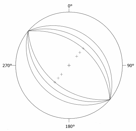
Alright then, what do we see here? For one of course the fold limbs, these are pretty easy to recognise; one is dipping towards North-East and the other one towards South-West. However, if you remember correctly, there is still something different, that we can see here. Could you already detect it? Yes, the fold axis! “Huh, where is the fold axis?” you might think to yourself right now. Well, the fold axis is always there, where the planes of a fold intersect to. This intersection is then visible in Schmidt’s net as a point and a point is…. a vector, correct! And what is the fold axis? A vector, too! Remember, a Schmidt’s net is the bottom side of a sphere. Therefor, if the intersection point of the planes is at the edges of the net, the resulting vector and therefor fold axis must be horizontal.
Got it? Good, because now you might be thinking: “A horizontal fold axis, how lame is that? I want something challenging!” Fear not, your wish will be granted.
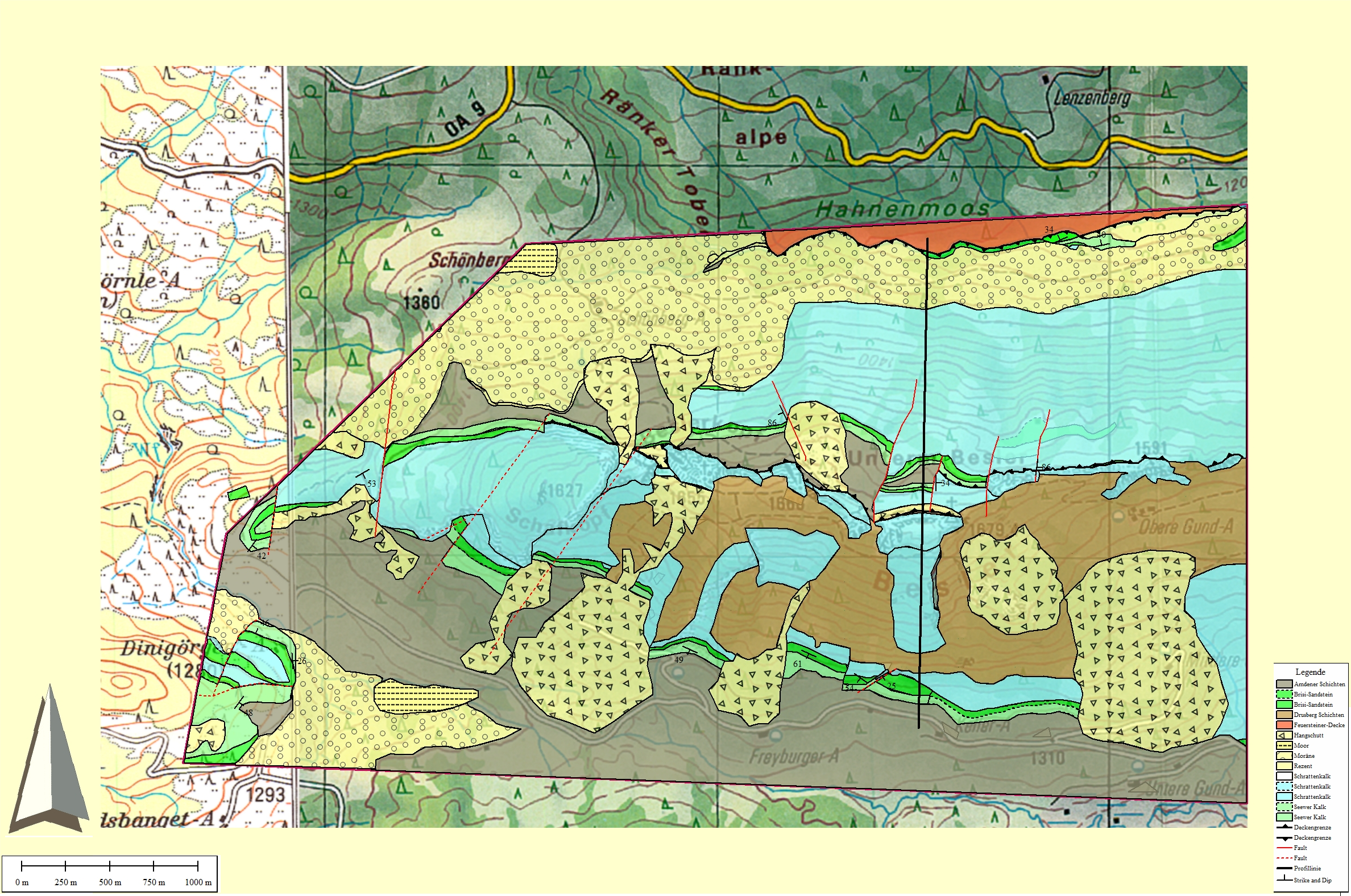
Why don’t we use a real-world example? Take a look at this map. There you can see a fold near Obermaiselstein in Bavaria, Germany that was mapped by a tag-team consisting of my mapping partner and, well… me. For now, all the intricate details do not concern us, just look at the Western part of the map. As you can see, the fold itself plunges down into the earth. As a result, the fold axis won’t be horizontal, but it will be… well; what will it be? To answer that question, you first have to take a look at Fig 2a.
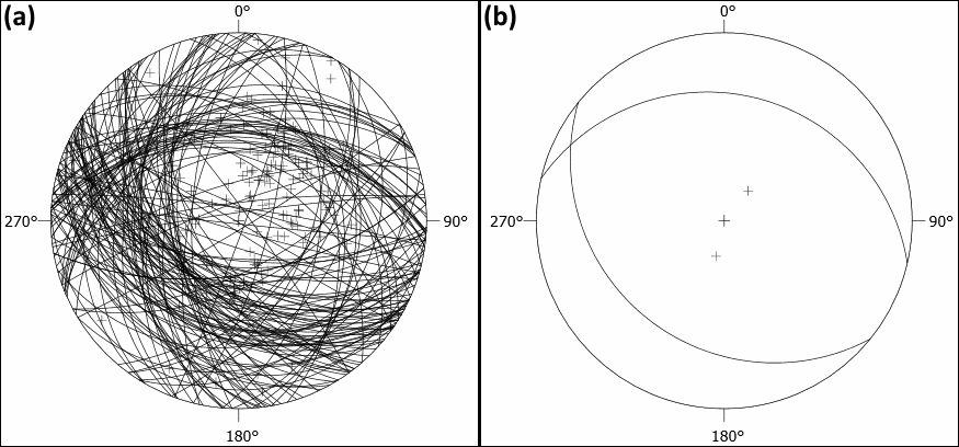
(a) display of all values
(b) display of the two resulting planes identified by cluster analysis
In Fig. 2a you can see all the directional values that we measured in the field. Quite confusing, right? How in hell are you supposed to see anything in there? Well, we only need two planes, one for each limb, right? So that’s what I did for Fig. 2b. By applying a cluster analysis and defining only two clusters we eventually end up with two planes with the following (Clar’s notation) values:
1: 013/22
2: 219/23
As you can see, the planes intersect at a point in the Northwestern part of the net. That means, that our fold is dipping westward (compare with map!) in our net. You can see that westward dip by the red square in Fig 3a (look below). Remember, the intersection vector of our planes is our fold axis. Therefore, the red point is our fold axis (a resulting axis plane will be tackled at a later point in time) with the values 296.3/05.3 in Clar’s notation.
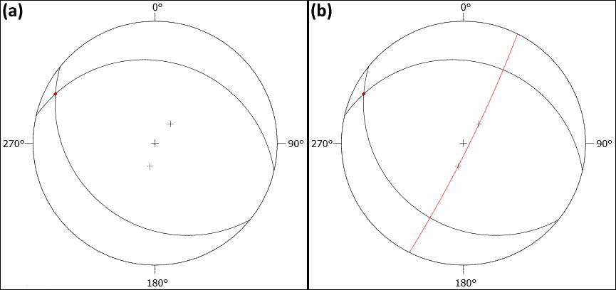
(a) marking of the fold axis. Dip value: 296.3/05.3
(b) the resulting π-circle with following values: 116.3/84.7
So…that’s it? Is that all, it is really that simple? Of course not, because now we are expanding a bit on that. Look back at Fig. 1. Do you see how the normal points of the planes all fall on one line? That is no coincidence. Remember the fold terminology: the plane that crosscuts the axial plane is called the profile plane and what do you get in Schmidt’s net, when you draw a line through several vector points? A plane, correct! Therefore, the normal points of the fold limbs create the profile plane. In fold analysis we call that one the π-plane or π-circle (Fig 3b). This plane can give us some field information: In the fold terminology I wrote that the π-plane is decoupling units of rock. Now take a look back at the map of the real-world example fold. Do you see how the main faults (meaning areas where blocks of stone have been moved relatively to each other; meaning units of rocks are decoupled) are more or less perpendicular to the fold axis? That means that the π-circle should incorporate the normal vectors of the planes and its normal vector should be where the fold axis is, right? And look at that, that is what is happening in Fig. 3b! Therefor the π-circle shows itself in the net with the measurements 116.3/84.7 (Clar’s notation). See, it all makes sense now: the π-circle is a representation of faults that are directly related to the folds.
What does that mean for you doing fieldwork? I mean, you won’t draw hundreds of planes into Schmidt’s net, right? Correct, that would be a waste of time. Instead when it comes to reconstruction, you only draw the bedding poles/normal vectors of you measured planes in Schmidt’s net. After having done this, you rotate your net until you find a great circle, that matches with your bedding poles the best. If you then draw a great circle using these bedding poles, you then have created your π-circle and if you have that one, you can also construct the fold axis vector. Oh, and don’t worry, if your measurements do not form one uniform line, it’s okay to have some outliers.
And there you have it, now you know the basic steps to reconstruct a fold in Schmidt’s net. Tune in next time and you will learn how to determine the opening angle of a fold.
All graphics created with Stereo32
Literature for further studying:
Lisle, R.J. & Leyshon, P.T. (2004²): Stereographic Projection Techniques for Geologists and Civil Engineers. Cambridge University Press
