As you can probably imagine, not all folds were created equal, especially when it comes to their opening angle. There are wide folds, tight ones, etc. Anyhow; how do we determine the opening angle of a fold? Well, if you want to know that, then just continue reading.
First and foremost, we are going to use the basis that we already established in the post about folds elements in Schmidt’s net. If you are new here, it could be helpful to read up on that first.
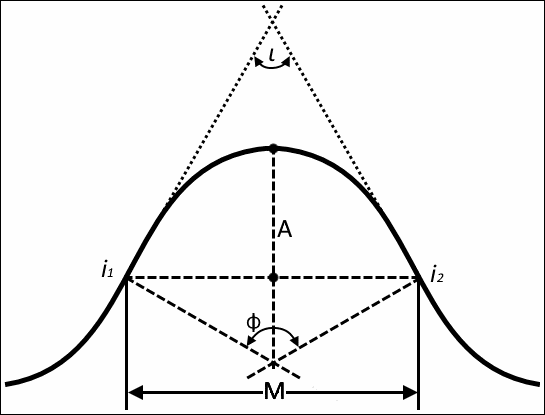
Alright then: What is the opening angle of a fold? Well, it is the internal angle of a fold. This angle is created between the two tangents lying on the inflexion points of a fold. Errr, sorry, what please? No need to panic, just look at Fig. 1.
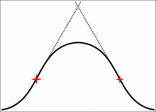
In Fig. 1 you can see a representative example of a profile through a cylindrical fold. On both sides you can find the so-called inflexion points (marked with red stars in the picture). That means that if we see the outline of a fold as a mathematical function, we can use the first derivate of the equation to calculate the tangent equations at the inflexion points (use of 2nd and 3rd derivate equation). Now, don’t panic here. I won’t torture you with “difficult” math, I just want you to understand the concept, alright? If we would to the calculation, we would eventually find two tangent equations, visualised here with the dotted lines. The opening angle is now measured as the angle between these lines.
However we do not want to calculate the opening angle. Instead we want to read that angle from Schmidt’s net. So, how do we do that?
First of all you need a π-circle. For that I used the one of the previous posts (to be clear; the orientation of the π-circle is like before but there are now some more planes in there!) and made some minor adjustments. You can see it in Fig. 2a.
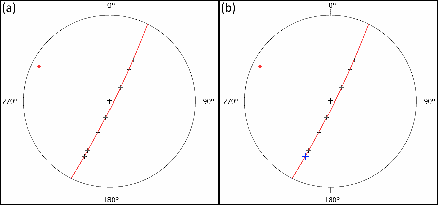
(a) Schmidt’s net with all used poles.
(b) The two outermost poles are marked blue. These represent the planes with the steepest dips, thus being the nearest to the inflexion points
As you can see there, I added some more normal points that create the π-circle (Remember, every point corresponds to a great circle/plane and these are your field measurements). So, you got a bunch of points and a π-circle, but how do you get any information about the opening angle from that? Well, think about earlier. What are features of an inflexion point in a function? At this point a function changes from concave to convex or vice versa and it is the point with the highest amount (meaning steepest) slope of a function. That means we have to find the planes with the steepest angles. And how are great circle and normal point related? Exactly, the nearer the first lands on the centre of the net, the further to the rim the second one will be situated. Thus, we need to find the points that are the furthest away from the centre on the π-circle. I marked them in a blue colour in Fig. 2b.
Now we need to rotate our net up to the point that the vertical axis of the net lines up with the π-circle (Fig. 3a).
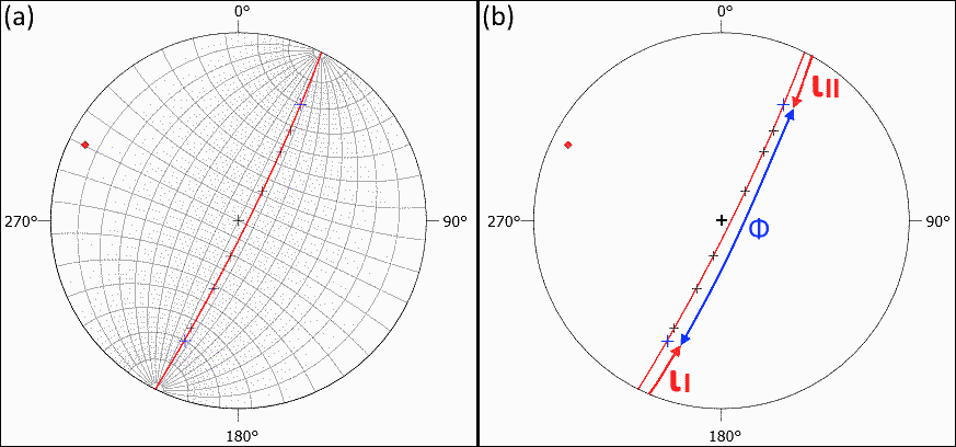
(a) the rotated net, so that the π-circle is aligned with the N-S-axis of the net.
(b) the two possible angles.
If we do that, we can simply count the angle between the points, however we now reach a little problem. As you can see in Fig. 3b, there are two possibilities regarding which angle we choose. We can either use the angle between the points (marked as Φ) or we can count going from the points to the outside (marked as ι). Depending on the situation we now get two angles, the acute (the smaller angle, in this case Φ) and the obstuse angle (the larger angle, in this case ι) but which one is the opening angle of the fold? In order to determine the opening angle, we always have to use the “outer” angle, in our case ι.
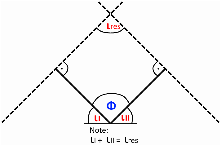
Why is this the case? Let’s use our imagination. A quadrangle always has an internal angle sum of 360°. Let’s imagine we create a quadrangle from out both tangential equations (“extended fold limbs”) and their normal vectors. A normal vector is always oriented 90° to its surface and since we have two of them, 180° are already gone. Meaning the angle between the limbs and the one between the normal vectors together add up to 180°. What also is divided into 180° in total? The N-S-axis of Schmidt’s net. Meaning, the angles between the poles (normal vectors) and the planes is both represented on the π-circle, when oriented in a vertical position. Now, what do we measure on that circle? The internal angle between the poles! As a result, the “outer” angle is our opening angle of the fold. So, how do we calculate the opening angle? Well, either we count the respective values of ιI and ιII in Schmidt’s net together in order to determine the overall opening angle ιres (res= resulting). Alternatively, and much less confusing: Just count the internal angle Φ and then solve the simple equation 180° = Φ + ι for ι (BEHERA, 2018; TWISS, 1988). In our example, the “internal” angle Φ of 140°. Thus, the opening angle ι in our example is 40°. If you need a visual representation of the whole problem, just take a look at Fig. 4.
See, that wasn’t that complicated, right?
Now there is only one thing to tackle. A simple number telling you the internal angle of the fold does not create an image in your mind, right? Therefor, some names were given to certain opening angles. As an example, I incorporated the classification after TWISS (1988) in table 1. Closely related to this is the aspect ratio of folds, meaning the ratio between their length and width. The respective terms can also be found in table 2. Finally, in Fig. 5 you can see all the different ratios packed into one graphic.
Table 1. Tightness of Folding (after TWISS, 1988)
| Descriptive Term | Folding Angle Φ, deg | Interlimb Angle ι, deg |
| Acute | ||
| Gentle | 0 < Φ < 60 | 180 ≥ ι > 120 |
| Open | 60 ≤ Φ < 110 | 120 ≥ ι > 70 |
| Close | 110 ≤ Φ < 150 | 70 ≥ ι > 30 |
| Thight | 150 ≤ Φ < 180 | 30 ≥ ι > 0 |
| Isoclinal | Φ = 180 | ι = 0 |
Table 2. Aspect Ratio (after TWISS, 1988)
| Aspect Ratio P | ||
| Descriptive Term | P = A/M | log P |
| Wide | 0,1 ≤ P < 0,25 | -1 ≤ log P < -0,6 |
| Broad | 0,25 ≤ P < 0,63 | -0,6 ≤ log P < -0,2 |
| Equant | 0,5 ≤ P ≤ 2 | -0,2 ≤ log P < 0,2 |
| Short | 1,58 ≤ P < 4 | 0,2 ≤ log P < 0,6 |
| Tall | 4 ≤ P < 10 | 0,6 ≤ log P < 1 |
And there you have it. Finally, after probably some dead brain cells you have mastered even this and now know how to determine the opening angle of a fold. Maybe I should have made a video about that instead, who knows.
Sources:
BEHERA, B. M. (2018): Basics of stereonet analysis Part – 2/3 by Prof. T. K. Biswal IIT BOMBAY. YouTube-Video. URL: https://www.youtube.com/watch?v=7AFmcT1uTBs. Last actualisation: 27.10.2019
TWISS, R.T. (1988): Description and classification of folds in single surfaces. Journal of Structural Geology 10/6
