In the previous post we covered the basics of stress and strain, but these alone are nothing. We need some examples! So; what are these? Obviously, I could talk about folds and faults now, but that is boring. Instead, let me introduce you to the Flynn diagram. We can use this in combination with our strain ellipsis to evaluate deformation regimes and therefor gather evidences for the development of a specific tectonic regime. Sounds interesting? Ok then; let’s go!
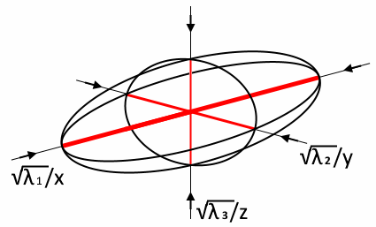
First a small reminder. What is the strain ellipsis? Well, the strain ellipsoid (Fig. 1) is the representation of the shape that a perfectly spherical grain would take if it was put in a defined stress regime. By convention the x-axis is always the axis of biggest elongation, while the z-axis gets the least elongated (meaning; in relation to the previously existing sphere it shrinks).
In order to illustrate the whole diagram to you, I will give you an example. Let’s say we find a rock with a bunch of ellipsoidal grains in it. In order to use the diagram, we now have to measure the length of the axes of the grains in our sample. (That means, that we have to note the orientation of the sample in the field before we even think about our hammer. Why? Well, because we want to determine the orientation of the stress field!)
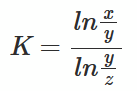
For our specific example the x-axis shows a length of 3 cm, the y-axis shows a length of 2 cm and the z-axis shows a length of 1 cm. Now, let’s think a moment. What would happen, if we would change these values? Maybe, let’s say make it so that y=x or y=z. Our ellipsoid would change its form, correct? Indeed; these would be completely different shapes that we would be able to see. Therefor, in order to classify these different shapes some parameters together with a diagram were thought of; the Flinn diagram (Unfortunately I was not able to track down the original source publication for that, so yeah; you will have to deal with that. If you know of the first instance, where that diagram popped up, please notice me!). In order to use that diagram, we first have to introduce a new parameter; K. This parameter is defining the style of strain, meaning: the shape that the ellipsoid takes. K is calculated with:
Now, there is a little thing that I have to highlight here. In many publications (and also up to this point in the introduction) you can see that e.g. λ1 is used similar to x. This is actually wrong, if one wants to use proper terminology, but it does not matter here (see this post coming soon for explanation).
As you can imagine, different lengths of the axes result in different shapes. With that knowledge we can now construct the Flinn-diagram. In the origin point sits an undeformed sphere. This sphere now gets deformed, resulting in a value for K. That K-value functions as the slope of a specific function (see further down) in the diagram. Therefore, the values of ln(y/z) plot on the x-Axis in the Flinn-diagram, whereas the values of ln(x/y) plot on the y-axis. In addition to that, the Flinn diagram also contains the D-value. This value classifies the amount of strain; the ellipsoidicity (meaning how far away the ellipsoid is away from a perfect sphere) of our deformed grain. D is calculated with:
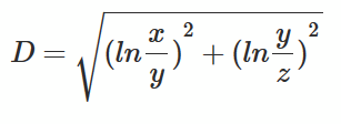
and represents the distance from the origin (meaning: perfect sphere) to your data point in the diagram. With all these values, we can now construct our Flinn-diagram (Fig. 2).
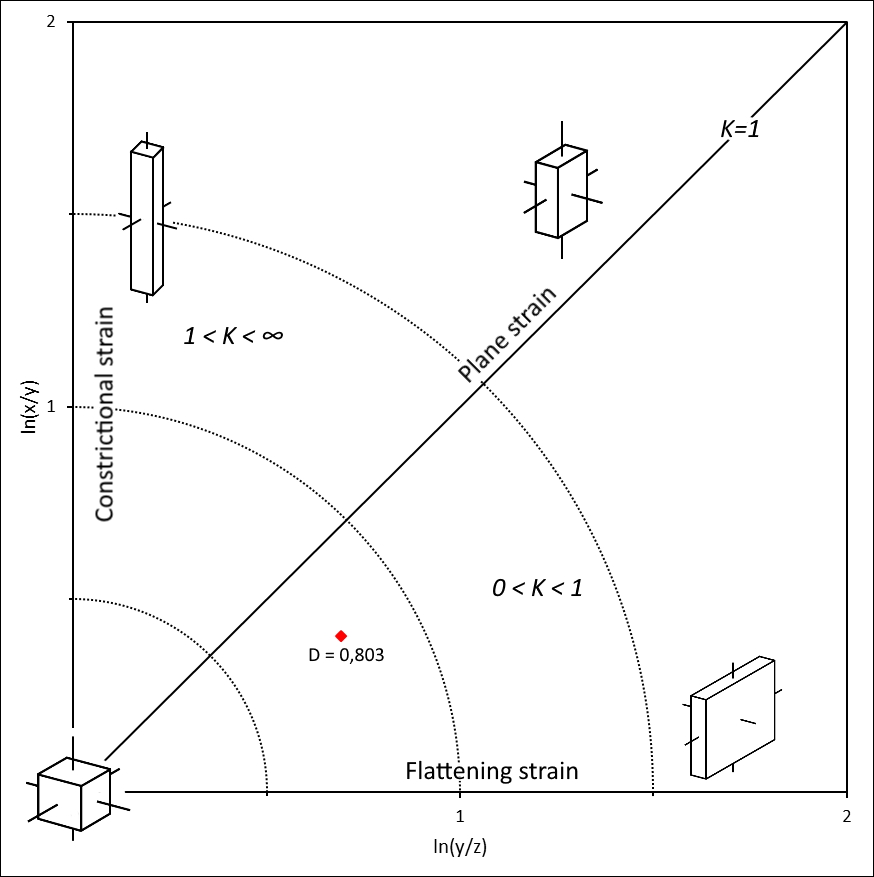
If you now take a look at the diagram, it won’t come as a surprise now if I tell you that the diagram can be differentiated into several sectors. These are based on the values for K:
| K –> ∞ | axially symmetric extension: x >>> y = z | the objects appear in a pencil-like shape and plot near the y-axis |
| ∞ > K > 1 | Constrictional strain: x > y ≥ z | the ellipsoids are elongated mainly along the x-axis, they look like cigars (so-called prolate ellipsoid) |
| K = 1 | plane strain deformation: x > y > z | all deformation happens in one (mathematical) plane, that is perpendicular to y. The y-axis does not change in its length |
| 1 > K > 0 | Flattening strain: x ≥ y > z | ellipsoids get flattened down mainly along the z-axis, they look like thick pancakes (so-called oblate ellipsoid) |
| K –> 0 | axially symmetric flattening: x = y >>> z | objects get extremely flattened only along the z-axis |
As you can imagine, the K-value as presented in the table (Tab. 1) only represents the theoretical shape that can be reached in the end. As how pronounced that shape is, that is determined by the D-value. In our case the D has a value of 0,803, meaning that our grain is relatively similar to a sphere. The stress regime therefor has been relatively low for that grain.
So, why do we need all that? Well, think back about the different types of shear. There was “pure shear” and “simple shear”, right? Now, let’s look at the Flinn-diagram. Do you think one can produce pancake-shaped ellipsoids when only simple shear is applied to a rock with uniformal grains to it? Nah, I don’t think so either, but with pure shear, that would work perfectly, right?
As a result, we can use the shape of deformed mineral grains to trace that back tectonic regimes. Especially metamorphic rocks are awesome for that. We call these tectonites, which will be covered in another post (coming soon).
Ressources
Rey, Patrice: Strain and Strain Analysis. In: Structural Geology. URL
Burg, Jean-Pierre: Strukturgeologie 2019 – Konzept der Verformung. URL
